TUTORIALS

Adiabatic heat bath Sod's shock tube Subsonic case 1. Case setup 2. Running 3. Solution 4. Regression testing Supersonic case 1. Case setup 2. Running 3. Solution 4. Regression testing Blunted cone RAM C-II spacecraft NASA MSL forebody Running your own case

☰

Sod’s shock tube

One-dimensional | AUSM⁺-up flux scheme

G. A. Sod, "A Survey of Several Finite Difference Methods for Systems of Nonlinear Hyperbolic Conservation Laws", J. Comput. Phys., vol. 27, pp. 1-31, 1978.

Subsonic case

Working directory located here

1. CASE SETUP

1.1 Mesh

The mesh is one-dimensional (empty patches for walls in the y and z directions) and a resolution of 10 mesh points per meter is used along x. Zero-gradients boundary conditions are implemented at both ends of the tube.

1.2 Case conditions

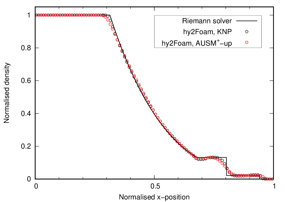
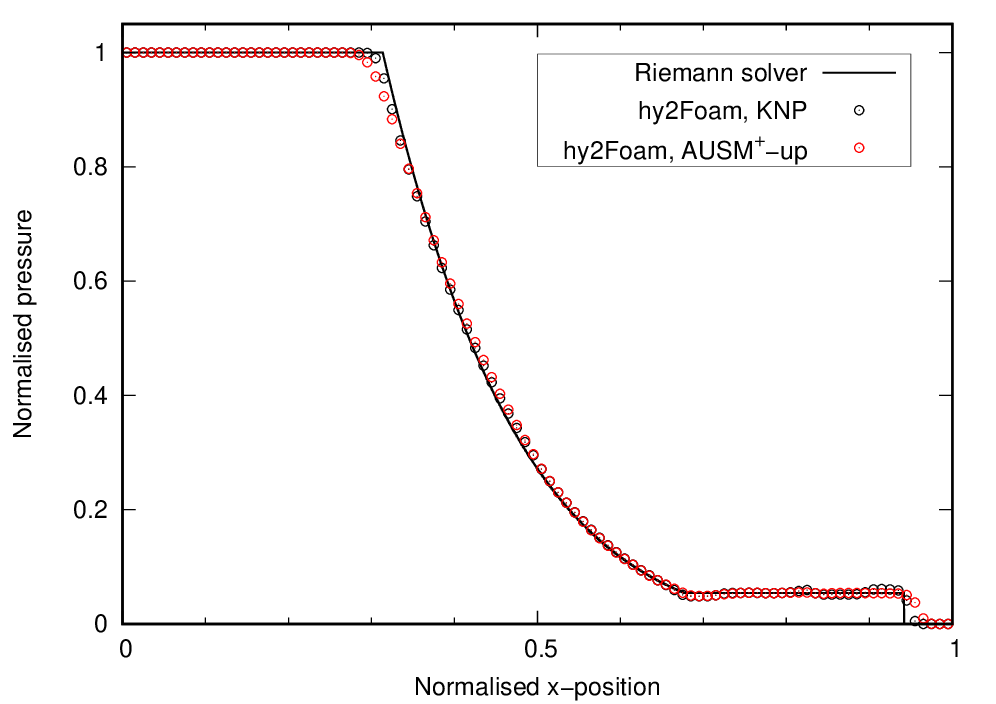
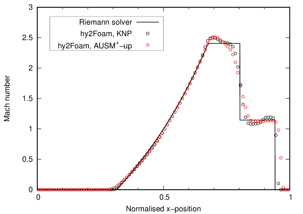
A one-dimensional subsonic Sod tube of length L = 10 m is considered with initial conditions for the left (L) and right (R) states chosen to match the normalised values presented in the following Table. These conditions should yield from left to right an expansion wave (E), a contact discontinuity (C) and a shock wave (S).

State	Normalised density	Normalised pressure	Mach number
Left (L)	1	1	0
Right (R)	0.125	0.1	0

The diaphragm located in the middle of the tube breaks at t = 0 s.

1.3 Thermo-chemical and transport models

This test case is using the following thermo-chemical and transport models:

calorically-perfect nitrogen gas
inviscid fluid
no chemical reactions
single-temperature model
laminar flow

1.4 Time controls

The constant time-step is set to 1 µs and the simulation is run until t = 5 ms.

1.5 Time and flux schemes

The temporal and flux schemes used are the first-order implicit Euler time scheme and the AUSM⁺-up flux scheme, respectively. The AUSM⁺-up model coefficients are given below.

fluxScheme            AUSM+up;

fluxSchemeCoefficients
{
    AUSM+upCoefficients
    {
        MachInf          1.0;
        
        alpha         0.1875;
        beta           0.125;
        sigma            1.0;
        Kp              0.25;
        Ku              0.75;
    }
}

2. RUNNING

The following commands will execute blockMesh, checkMesh, setFields and hy2Foam in serial

./Allclean  
./Allrun

3. SOLUTION

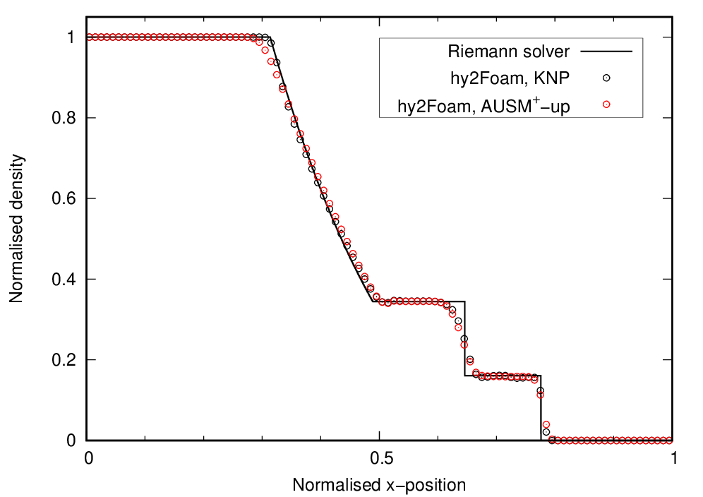
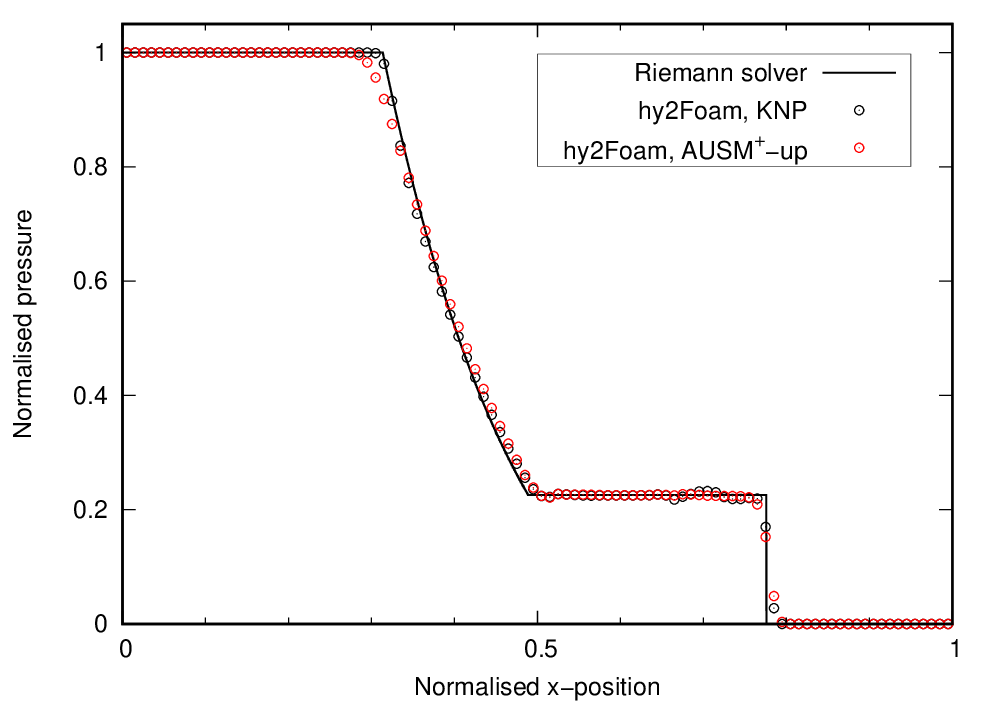
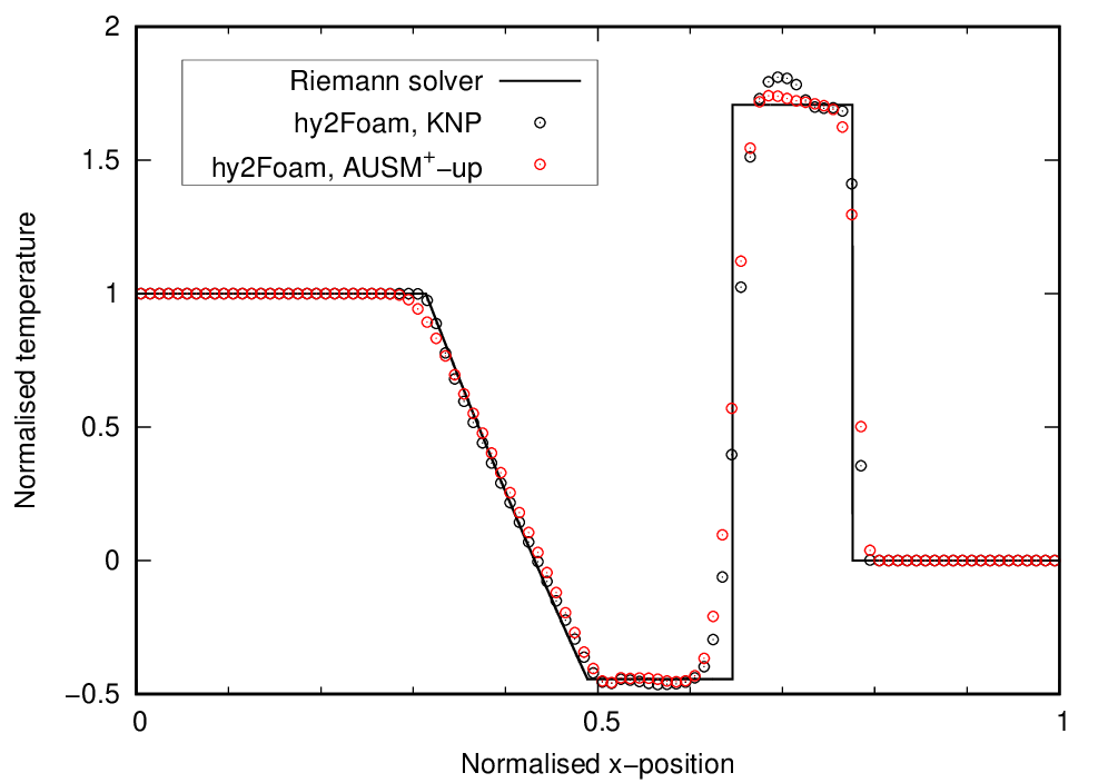
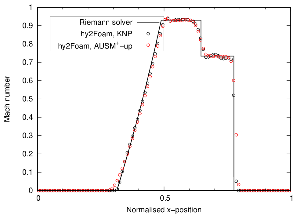
Length, density, pressure, and temperature are normalised as follows:

`x^∗ = \frac{x}{L}`,

`ρ^∗ = \frac{ρ - ρ_R}{ρ_L - ρ_R}`,

`p^∗ = \frac{p - p_R}{p_L - p_R}`,

`T^∗ = \frac{T - T_R}{T_L - T_R}`.

On the following graphs, the tutorial case results for density, pressure, temperature and Mach are given by the red symbols. hy2Foam’s solution for the Kurganov-Noelle-Petrova (KNP) scheme is also shown as a reference.

4. REGRESSION TESTING

Check that the results are matching the solution stored in gnuplot/solution/:

./Alltest

Supersonic case

Working directory located here

1. CASE SETUP

1.1 Mesh

See subsonic case.

1.2 Case conditions

The shock tube case introduced in the previous section is simulated again for a different set of initial left and right state conditions resulting in a supersonic flow:

State	Normalised density	Normalised pressure	Mach number
Left (L)	1	1	0
Right (R)	0.01	0.01	0

2. RUNNING

The following commands will execute blockMesh, checkMesh, setFields and hy2Foam in serial

./Allclean  
./Allrun

3. SOLUTION

Because the left and right temperatures are equal, the normalised temperature is computed as

`T^∗ = \frac{T - T_R}{T_R}`.

On the following graphs, the tutorial case results for density, pressure, temperature and Mach are given by the red symbols:

4. REGRESSION TESTING

Check that the results are matching the solution stored in gnuplot/solution/:

./Alltest

Contributor: Dr Vincent Casseau