
☰
Blunted cone
Axially-symmetric mesh | Thermal non-equilibrium | Slip boundary conditions
![]() Working directory located here
Working directory located here
![]() See Section 3.1. Mach 11.3 Blunted Cone in
See Section 3.1. Mach 11.3 Blunted Cone in
V. Casseau, D. E.R. Espinoza, T. J. Scanlon, and R. E. Brown, "A Two-Temperature Open-Source CFD Model for Hypersonic Reacting Flows, Part Two: Multi-Dimensional Analysis," Aerospace, vol. 3, no. 4, p. 45, 2016 [Full HTML→]
1. CASE SETUP
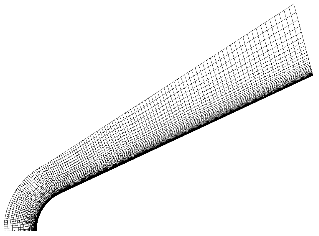
1.1 Mesh
View of the structured gmsh mesh provided in the
1.2 Case conditions
The blunted cone is a fully-diffuse surface set at a temperature of 297.2 K. The inert fluid is N2 and the freestream conditions are given in
- Ma∞ = 11.3
- Knov = 0.002
- p∞ = 21.9 Pa
- Ttr, ∞ = 144.4 K
- Tv, ∞ = 144.4 K
- U∞ = (2764.5 0 0) m/s
Smoluchowski temperature jump and Maxwell velocity slip boundary conditions are used.
1.3 Thermo-chemical and transport models
This test case is using the following thermo-chemical and transport models:
- thermally-perfect gas (excluding the electronic energy contribution)
- no chemical reactions
- two-temperature model
- V—T energy transfer: Landau-Teller, tabulated Millikan-White coefficients, Park’s correction
- species viscosity: power law
- species thermal conductivity: Eucken
- laminar flow
1.4 Time controls
The initial time-step is set to 1 x 10⁻¹⁰ s and the maximum CFL number is 0.5. The simulation end time is equal to 0.0002 s.
2. RUNNING
The following commands will execute gmshToFoam, checkMesh and hy2Foam in serial
./Allclean
./Allrun
To run hy2Foam in parallel (say on 4 CPUs), please first edit the
./Allclean
./Allrun 4
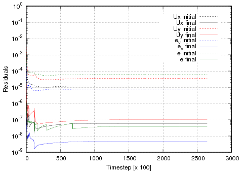
3. MONITORING
gnuplot gnuplot/monitorResiduals
4. FLOW VISUALISATIONS IN PARAVIEW


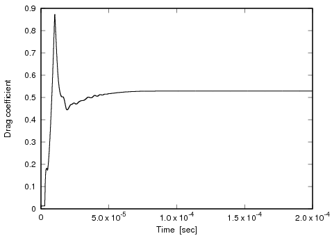
5. POST-PROCESSING
gnuplot gnuplot/monitorCd
gnuplot gnuplot/monitorIntegratedWallHeatFlux

6. SOLUTION
On the following graphs, the tutorial case results are given by the black solid lines:
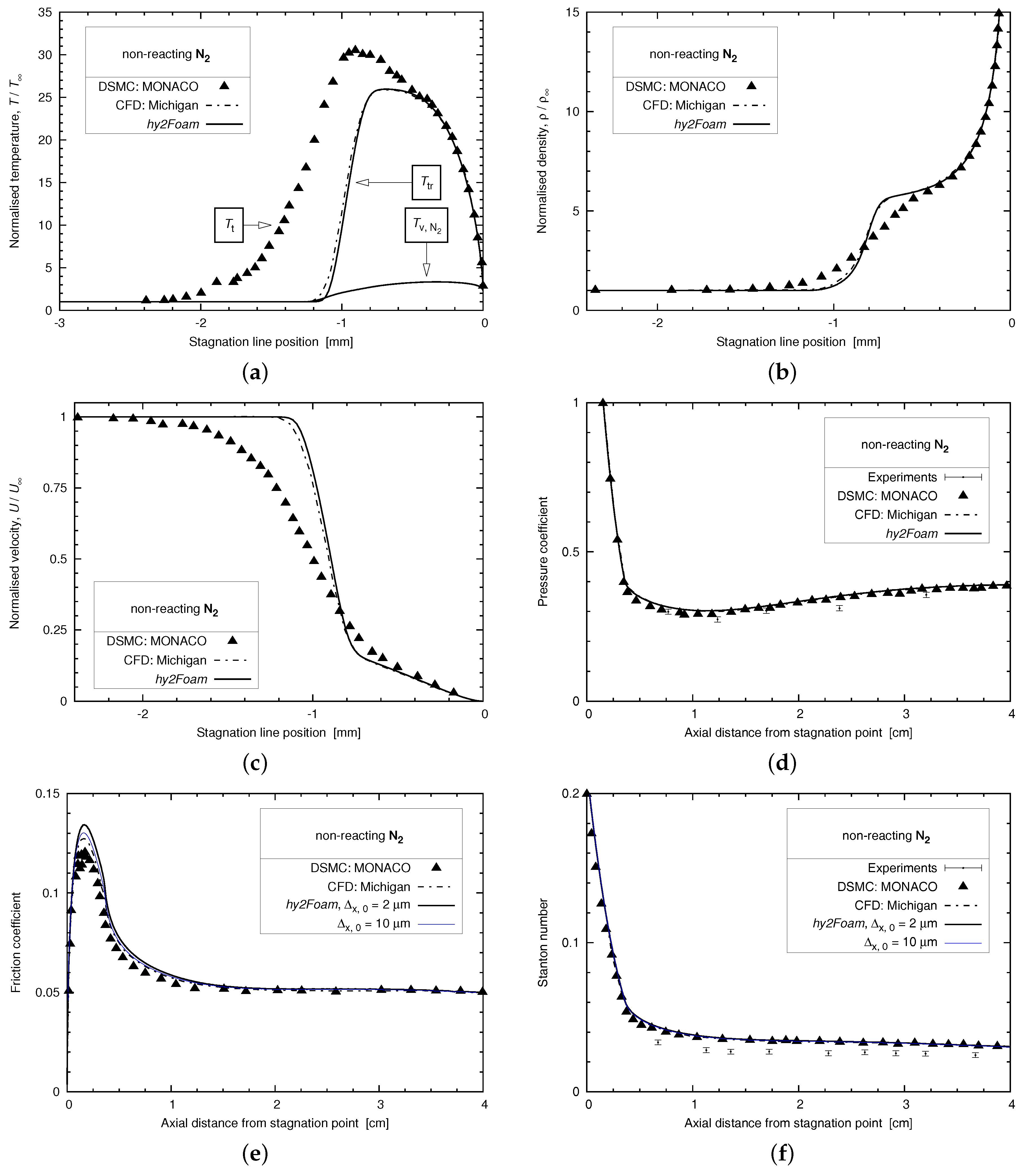
Stagnation line data (a–c) and surface coefficients (d–f) along the blunted cone:
(a) normalised temperature, (b) normalised mass density, (c) normalised velocity, (d) pressure coefficient, (e) friction coefficient, and (f) Stanton number.
7. REGRESSION TESTING
Check that the results are matching the solution stored in
./Alltest
Contributors: Dr Vincent Casseau and Dr Daniel E.R. Espinoza